Dependent Drop Down Box

How to do one of those trickier tasks in Excel: set up a drop down box that is dependent on the result of another drop down box.

The scenario

If coffee is selected from drop down A then I want a list of coffee types to appear in drop down B. If Tea is selected in drop down A then I want a list of tea types to appear in drop down B.

In the real world these lists may be product type and sub-products, departments and employees, account groups and sub accounts etc.

I’ve saved a file here for you to download and see how I’ve done it.

 

 

Step 1: Set up your primary and secondary tables

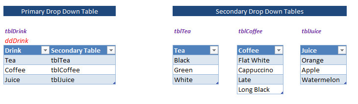
Note how the primary table has a column containing the names of the associated secondary tables

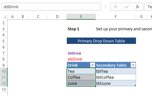
Step 2: Set up your Primary Drop Down List called ddDrink

To do this highlight the 3 cells Tea, Coffee, Juice and go to the Name Manager Box above column A and type ddDrink and then press Enter

 

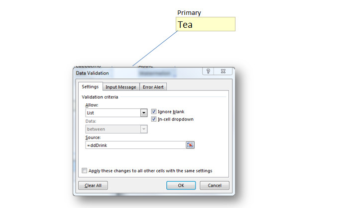
Step 3: Set up your Primary Drop Down box

Click on a cell, lets say G21 and select Data > Validation > From List and type =ddDrink in the source box

Step 4: The trickier bit : Set up your Secondary Drop Down list

Here’s the trickier part

Let’s say we want our secondary drop down box to be right next to our primary drop down.

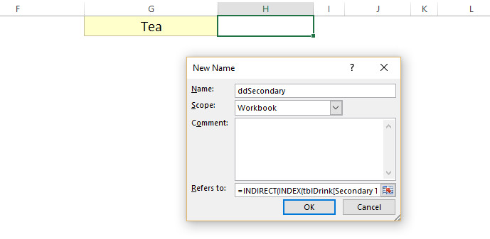
So we click on cell H21, and now we are going to create a named range called ddSecondary

To do this, click on Formulas > Define Name and name it ddSecondary

then add this formula to the Refers to: box

=INDIRECT( INDEX( tblDrink[Secondary Table],MATCH( G21, tblDrink[Drink],0)))

That’s a pretty nasty looking formula when looked at in one go.

Ignoring the INDIRECT part for a moment, the main element is an INDEX MATCH formula which I’ve written numerous articles on and even made a video about.

The INDIRECT part is the “clever bit” in that it indirectly gives you the table name to be used for the second drop down.

For example, if Tea is selected in G21 then the INDEX MATCH part looks up the word Tea in the Drinks Table and then returns the corresponding Secondary Table name of tblTea.

The INDIRECT part then uses the reference to tblTea to provide a list to be used by the Secondary Drop down box.

Not easy to understand on first pass, Give it a try and feel free to ask for help.

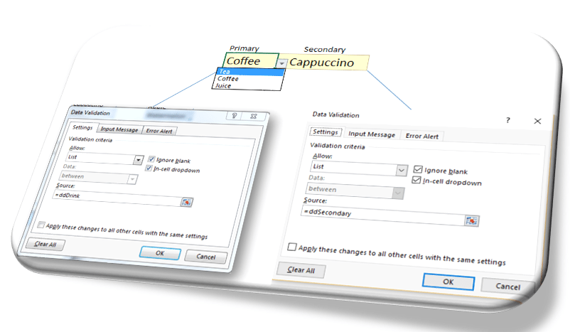
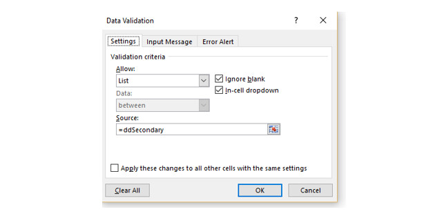
Step 5: Set up your secondary drop down box

Click on cell H21and select Data > Validation > From List and type =ddSecondary in the source box

Step 6: You’re done!

A very useful extra step is to add conditional formatting to flag invalid combinations such as Flat White Tea or Apple Coffee

To see how I’ve done that take a look at the demo file, essentially I use a COUNTIF formula in the conditional formatting.