Spreadsheet Detective FeaturesSpreadsheet Detective | Features | Free Download | Pricing | Spreadsheet Auditing |
Basic Features
- Workbook Report
- Audit Excel Formulas with Shading
- Map Report
- Excel AutoName Formula Report
- Full Annotations
- Data Flow Interactive Task Pane
Advanced Features
- Comparing Spreadsheets
- Audit Process Control
- Worksheet Interactive Task Pane
- Worksheet Data Flow Report
- Master Key Encryption
- Precedent/Dependent Reports
- Workbook Discovery Report
- Manipulating Named Ranges
- Sensitivity Report
- Other Features
Content and images below provided courtesy of The Spreadsheet Detective.
Download a free 60-day trial, then purchase The Spreadsheet Detective through Access Analytic for a 5% discount, or contact us for further information about our Spreadsheet Auditing Services.
Workbook Report
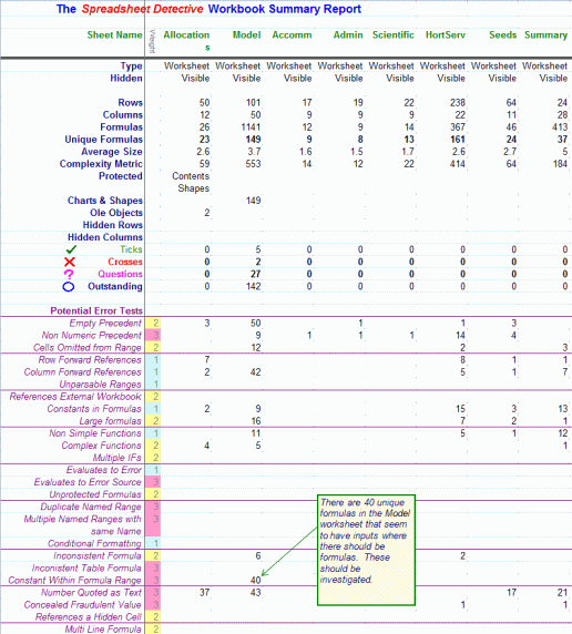
The workbook summary report provides an overview of every worksheet in a complex model. The first section lists each sheet in its own column, together with basic statistics such as how large the worksheet is and how many distinct (unique) formulas there are.
It also shows hidden and very hidden sheets. (These can be unhidden using the new Worksheets Pane).
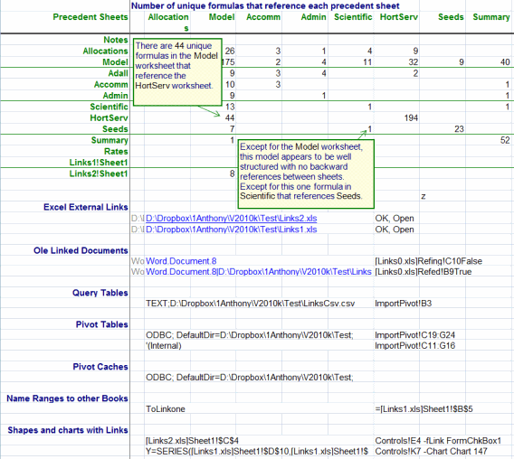
The third section is perhaps the most important because provides a comprehensive overview of the data flow within a model. It does this by showing the number of distinct formulas in each sheet that reference cells in other worksheets.
In this example there are 44 unique formulas in the Model worksheet that access the sheet shown.
The final section documents all external links to other objects in detail. Some of the links can be very frustrating to find without the Spreadsheet Detective when Excel reports that there are links to other workbooks.
Audit Excel Formulas with Shading
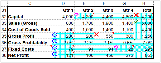
The Spreadsheet Detective has automatically added blue shading to all cells that contain a formula. This makes it clear that G35 does not contain a formula which is why the total in I38 is wrong.
Horizontal stripes indicate that the formula has been copied from the formula to the left, while vertical stripes indicate that the formula has been copied from above. This highlights the fact that that the formula in cell H37 is inconsistent with that in cell G37.
By default cell notes/comments are also added that use AutoNames such as “`Sales” to describe each unique formula as shown for cell E35. These are described in detail in the AutoName Formula Report below.
Excel has used green triangles to highlight cells such as I32, which it thinks has errors in them. However, the result is not very satisfactory. Many valid constructs are flagged as erroneous while important errors are overlooked. In the example spreadsheet, Excel has flagged four valid cells as wrong but none of all seeded errors have been detected.
These errors could easily be overlooked without the Spreadsheet Detective.
Map Report
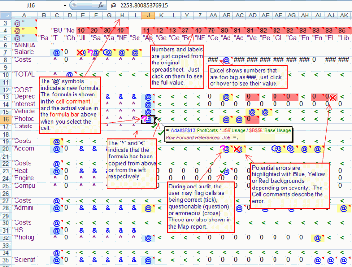
The map report shown above makes it easy to see the structure of larger worksheets.
Like earlier Shaded option, it shows how formulas have been copied, and cell comments describe the formulas with AutoNames. However, unlike the Shaded option the results are placed on a newly created, separate report worksheet.
They are also condensed which makes it easier to understand large worksheets.
In the cells, “@” means new formula, “<” means copied from left, “^” means copied from above, and “&” corresponds to speckled. “###” is just Excel’s normal way to show numbers that are too wide to fit in the narrow columns.
The original values of the formulas are placed to the right of the symbols, and so can be seen in the formula bar by simply selecting a cell, or by making a column wider. Excel also enables large numbers to be seen simply by hovering the mouse over a cell.
Potential errors found by the Spreadsheet Detective are included in the cell comments, and the cells are coloured to provide a heat map of potential issues. The Audit Process Control may flag cells as being correct, questionable or dubious and these are also shown on the map with ticks, question marks and crosses respectively.
Excel AutoName Formula Report
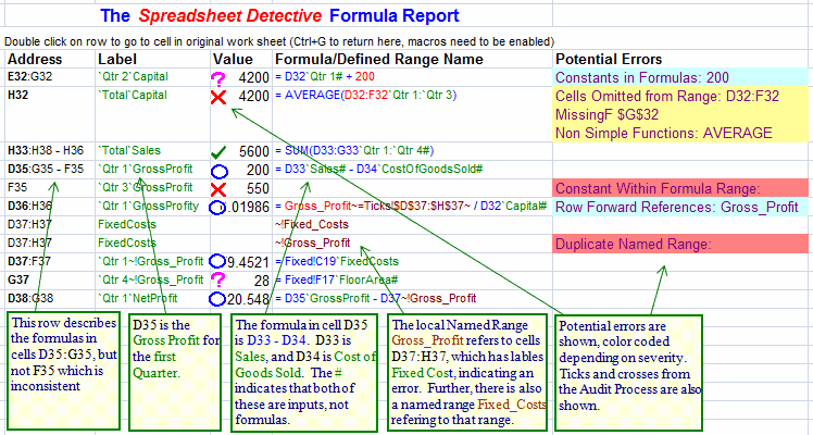
The Spreadsheet Detective can create a report of all formulas in a spreadsheet. Note that only the distinct formulas are listed which greatly reduces the number of formulas that need to be reviewed.
The cells containing the formulas are indicated using both A1 references in the first column and with AutoNames in the second column. Thus it is clear that cell E35 is the first Quarter’s Gross Profit. The notation also shows the formula has been copied into cells E35:H35, but with the exception of cell G35, again highlighting the error.
The formula is then displayed with AutoNames again interspersed with the A1 references. This makes it easy to verify that they are referring to the correct cells. There are several other notations, for example the “#” indicates that the precedent cell E33 is a simple input, it does not contain a formula.
AutoNames are automatically derived from labels on the worksheet.
Sophisticated heuristics are used to identify the correct cells to use, they do not have to be in any particular row or column. It is also possible to override AutoNames where necessary. AutoNames are an essential tool for understanding and verifying A1 references, particularly to more distant cells.
The value of the first cell in each range is also listed as a convenience. The report includes any named ranges that refer to cells on the selected worksheet. In this case the local named range Gross_Profit refers to cells E37:I37, which has the AutoName FixedCosts. This makes it easy to see that the named range has been defined incorrectly.
Any potential errors found by the Spreadsheet Detective are also shown, together with ticks and crosses derived from the Audit Process Control. Double click on a row in the report to go directly to the cells in the original workbook.
Full Annotations
Full annotations also enables “A” lines to graphically show the range of aggregates which makes it easy to verify that the Code has not been accidentally included in the Average in cell I32.
However, the main advantage of this format is that the formulas to be shown on the worksheet itself rather than as cell comments. They show the original formula in blue with additional information in green and brown.
AutoNames are used to clarify the meaning of cryptic “A1” references. Thus the reference to cell E34 has been shown as “E34`CostOfGoodSold” because “Cost of Goods Sold” is the label in cell C34. Automatically including labels with formulas makes cryptic A1 references like “E34” much easier to understand and validate on larger models.
The annotation in C37 makes it easy to see that the Gross_Profit named range is wrong, which means that the reference to it in cell E35 refers to the wrong cell. It is very difficult to detect named range errors without the Spreadsheet Detective.
Data Flow Interactive Task Pane
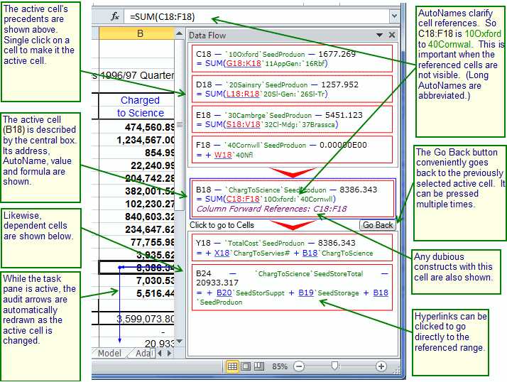
In Excel 2007 and later versions, the Precedent/Dependent Task Pane (above) shows the active cell’s formula & makes it easy to view a cell’s Precedents and Dependents.
The middle box describes cell B18, its AutoName, value and formula. The boxes above show the precedents, i.e. cells upon which B18 depends. The boxes below show cells which depend on cell B18. Again, the AutoName, value and formula are shown. A scroll bar appears if there are too many to display.
When enabled, the task pane automatically updates itself as the user moves around their model. The task pane can be disabled by simply closing it with the X on its top right.
Clicking on the precedent or dependent boxes selects the corresponding cell which then moves it to the central box. Its precedents and dependents can now easily be seen, following the chain from inputs to final results and back again. The Go Back button conveniently goes back to the previously selected cell. This provides a very effective method to navigate throughout a complex model.
The cell in the central box is always selected and made visible in the underlying workbook so that you can easily see its context.
Comparing Spreadsheets
This worksheet has been modified and then compared with the original worksheet.
The triangle symbol in E35 indicates that the Gross Profit formula has changed, while the “E” symbol in row 38 shows that these values are new because this row has been inserted.
The heavy dashed vertical line indicates that column G (Qtr 3) had been deleted.
Changes are only marked for cells with formulas if the formula changes.
Thus cell F39 has not been marked as being different even though its calculated value has increased from 4.5% to 6.4% because the formula has not changed.
This is important because one small change in an input value can change the values of many calculated cells which can make it difficult to see the underlying cause.
It is important to be able to compare a draft with a final version to ensure that new errors have not been introduced.
It can also substantially reduce the time required to check a new version of a model.
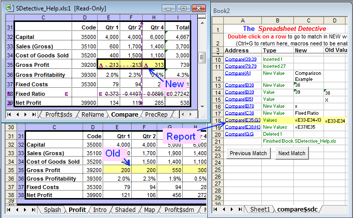
The comparison report lists all changes, and shows the New, Old and changes in one display. The changes can then be reviewed one by one by double clicking on the report rows.
Audit Process Control
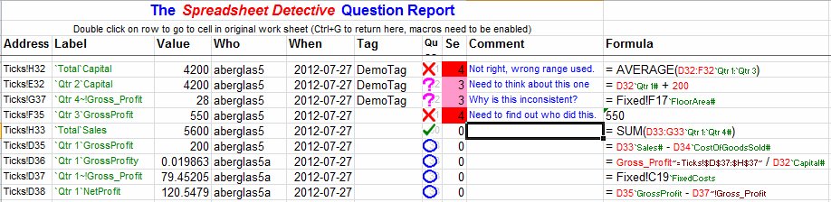
The Audit Process Control system enables cells to be manually marked as Verified (a tick), Erroneous (a cross), Questionable (a Question Mark) or Outstanding (a circle).
In the above example, F35 has been marked as Erroneous, E32 as questionable, and D35:D38 as Outstanding and so not yet reviewed.
The Questions Report below then lists all the cells in the entire workbook that have been marked.
The report lists the cell address (with AutoNames), the severity, tag, date and time the mark was created, and any comments that were entered against the cell.
Cells are sorted by severity and also by a Tag optionally entered by the user, so that cells with the same tag appear together in the report even if they are in different worksheets.
The marks are also listed in the formula report and map report. The latter provides a solid graphical summary of where issues are.
Being able to accurately monitor the completeness of an audit and provide accountability is an important part of a process quality strategy.
Worksheet Interactive Task Pane
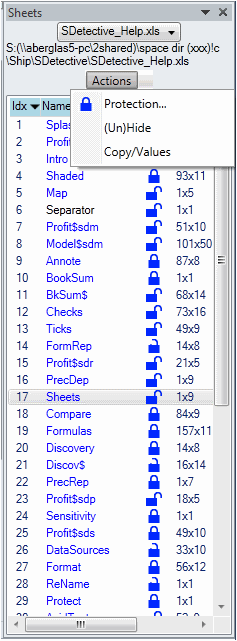
The Worksheets task pane provides a concise list of all the sheets in a workbook.
It is available in Excel 2007 and later. Clicking on a sheet selects that worksheet.
This can be very useful for workbooks that contain numerous worksheets as many more can be displayed in a vertical list than in tabs at the bottom of the page. Multiple sheets can be selected using Ctrl and Shift clicks in the normal way.
All sheets are shown, including Hidden (in black) and Very Hidden ones (in grey). Size is shown as the number of used columns and rows.
The padlock indicates that a sheet is fully protected, unprotected, or partially protected.
The list can be sorted by Name, size (i.e. total number of cells), protection status etc.
Columns to the right (not shown) indicate the type of sheet and visibility status.
The top of the pane provides an easy way to select different workbooks. The books full path is then displayed. This includes the full, UNC name for any mapped drives in parenthesis.
Commands have been added to process multiple worksheets at once, such as changing their protection.
It is also possible to create snapshot copies of just a sheet’s values, and to create difference worksheets that show which cells have changed value between a snapshot and the original sheet.
Worksheet Data Flow Report
Full annotations and shading provide a detailed view of formulas in the small.
The worksheet data flow report provides a powerful summary of complex spreadsheets in the large.
The report is a Pivot Table that describes the number of unique formulas that reference cells in each worksheet.
Thus the Vincent worksheet contains two formulas that reference cells in the Trimix worksheet. This is of concern because a well designed model should have a clear flow from input sheets to output sheets but the Trimix worksheet also has six formulas that reference the Vincent worksheet.
The report is an ordinary pivot table so double clicking on a cell will drill down to show the individual formulas that are doing the referencing. The totals on the right show the total number of unique formula references within each worksheet which is an excellent metric of the sheet’s complexity.
The rightmost columns show references to worksheets in different workbooks. This compliments the inter workbook summary report which provides an even higher level overview of which workbooks call other workbooks.
Master Key Encryption
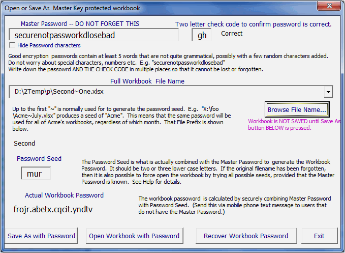
You deal with extremely confidential data. You have read about hackers breaking in, security being compromised.
You need to show your clients that you take security seriously.
You need to encrypt your workbooks. But what happens when you loose or forget the password?
People leave, minds forget. Last year’s forecast model is locked with an unknown secure password. It is Gone. Excel 2007+ is (finally) secure by default. Lose the password, you’ve lost the workbook.
The Spreadsheet Detective addresses this by enabling you to use a unique password for each workbook, and then a Master password that controls the individual workbook passwords. Clients can be safely given the workbook passwords.
As long as you do not forget the Master password, your workbooks are both protected and safe.
There would normally be just one master password for a department, which rarely changes. This may not be quite as secure as having a full, expensive and error prone key management system, but it provides much greater security than not using passwords at all.
Each individual (set of) workbooks has its own unique strong password, which is generated by the Detective.
This can be sent to people outside the department using a different channel such as a mobile phone text message.
They can then access the spreadsheet, but have no access to the master password or other workbooks protected by it (If the original workbook name is lost then its password can be recovered by the Spreadsheet Detective but only if the master password is known.)
This simple system does not rely on complex password servers which would need to be set up and managed by IT, and to be available whenever you need to access the spreadsheets.
Precedent/Dependent Reports
The precedent report describes how the Profitability cell (D37) was calculated.
The report lists the formula in D37, then the precedent cell referenced by it, and then the precedents of those cells recursively.
Note that cell Profit!D35 refers to Fixed!C19, and so row 13 of the report describes formulas on the Fixed worksheet.
Being able to see inter-sheet calculations is particularly useful when analyzing complex models that contain multiple worksheets.
The report is an outlined spreadsheet, and so clicking on a “+” or “-” will expand or collapse a set of precedents respectively.
Double clicking on a line within the report will go to the corresponding cell in the original worksheet.
Pressing Excel’s normal F5 function key will return to the report.
Note the way that the “#” makes it clear which referenced cells are input values and so avoids the need to look at those referenced cells explicitly.
Other reports show all the unique formulas in a given worksheet, and highlight potential problems such as references to non-numeric cells and unprotected formulas.
There is also a Dependent report that works in an analogous manner.
Workbook Discovery Report
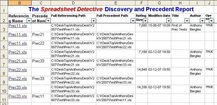
The Workbook Discovery and Precedent report helps discover where spreadsheets are located within your organisation, and how they relate to each other.
The report is produced in two phases. The first discovery phase scans a folder and optionally its sub folders for spreadsheet files. This can be repeated multiple times if necessary to scan different folders.
The second precedent phase opens each of the spreadsheets to determine their precedent worksheets as well as their Excel properties such as their title. A row is added to the report for each precedent that is found. Optionally the report can also recurse through any precedent workbooks that were not found in the original discovery scan.
The report can then be sorted to highlight either workbook precedents or workbook dependents. So in the example we can see that Prec11.xls references Prec21.xls and Prec22.xls, and that Prec21.xls references Prec33.xls etc. Thus the report provides a flexible and powerful view of all of the spreadsheets in an enterprise, and the relationships between them.
Manipulating Named Ranges
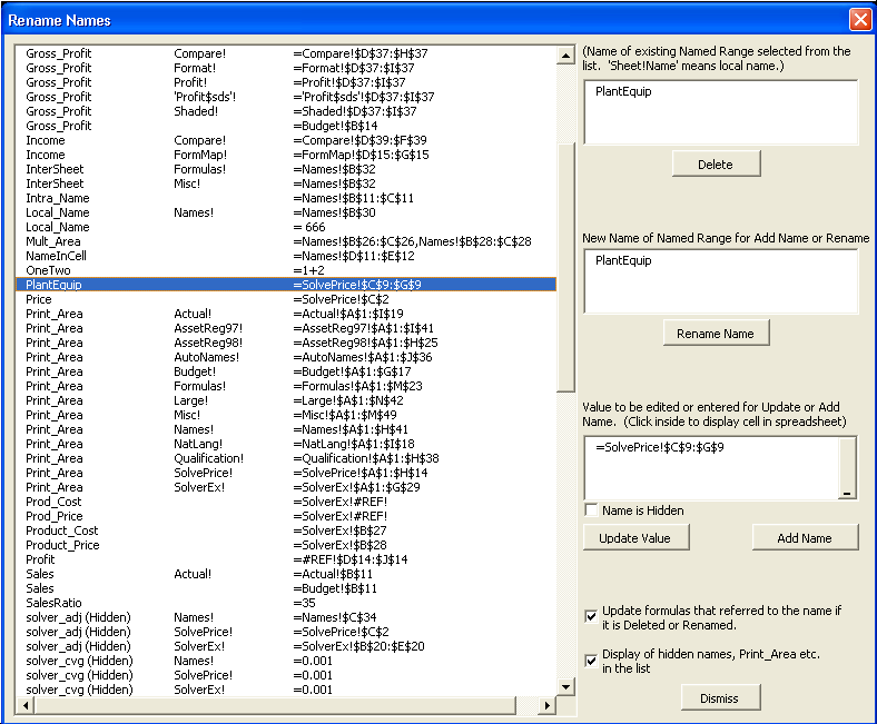
While the Spreadsheet Detective’s AutoName facilities reduce the need for Named Ranges, they are still useful for commonly referenced fields.
Excel makes it easy to create Named Ranges, but provides very little assistance with changing their definitions as the structure of a model changes.
The Rename Names feature enables a Named Range’s name to be changed and provides explicit information about local, global and hidden Names.
More importantly, the Detective can automatically update all the formulas that used the Named Range that has been renamed.
The generous dialog box shows all details of all Named Ranges including local and hidden Names.
These can be very confusing without the Spreadsheet Detective.
(This is no replacement for showing named range definitions right on the worksheets they refer to as is done in the Shading and Full Annotations.)
Sensitivity Report
The Sensitivity Report shows how sensitive a selected output value is to all the input values. The report is produced by replacing each constant or formula with a constant that is 10% (say) larger than its current value. The difference in the output value is then recorded in the corresponding cell in the report before the original value or formula is replaced and next cell selected.
Thus the above report shows that the Profitability is 63% sensitive to Qtr1 Sales, but is not sensitive to Qtr3 Sales. This highlights the error in the formula in cell G35.
Sensitivity analysis can produce a much deeper understanding of a model and can highlight many types of errors that are not obvious from absolute values.
Other Features
- Identification and separate listing of formulas that reference other workbooks
- Inter-Workbook Dependency
- Report that shows how multiple workbooks are (or are not) related
- Flagging of cells that ae (not) referenced by any unique formula
- Highlighting of formulas copied between different worksheets in three dimensional models
- Accurate documentation of complex local named range relationships
- Accurate visualisation of array formulas
- Highlighting of certain dubious constructs and circular references
- Documentation of charts
- Mechanisms to control and override AutoNames