
Easy Cumulative totals in Tables
The single greatest advancement in Excel in the last 10 years was the introduction of Tables. Yet although Tables were introduced in Excel 2007 there is still a huge number (I’d even say the majority) of Excel users that don’t know how to create tables or understand what they do.
This is a brief introduction
Click in a cell in a block of data (to be super safe highlight the entire block)
Press CTRL + T
Ensure that My Table has headers is ticked, and press OK
You now have a Table. There are 10 or so great features of Tables but here are the 3 key ones for me…
- Tables expand automatically when you type at the bottom or to the right. This is fantastic for those using Pivot Tables or Data Validation.
- Formulas “auto-fill” up and down the table whenever you enter a new formula or amend an existing one.
- INDEX MATCH works brilliantly with Tables
If you’ve never used Tables but you do use Excel to analyse “tables” of data then you are missing out on a huge opportunity
Cumulative Totals in Tables
One frustration I do have though is that cumulative totals in tables in a column are not straightforward.
In “normal” Excel to get a running total you just add the cell above to the cell on the current row, and that’s it.
For a table, with its structured references and headings this proves problematic.
Also, ideally you want a running total that works when you insert rows into the Table or add lines of data to the bottom of it.
So here are 3 options:
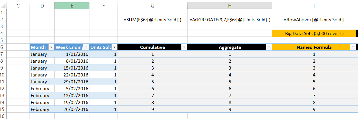
Option 1: If the heading of the Units Sold column is F6 then use =SUM(F$6:@
Option 2: A little more advanced since the SUM approach has a drawback.
If you filter the table for February you still get the YTD cumulative rather than just the February Cumulative
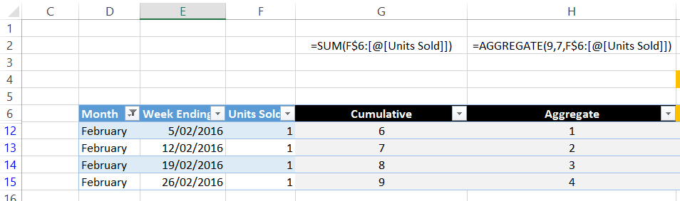
An alternative is the little known AGGREGATE function (you could also use SUBTOTAL).
=AGGREGATE( 9, 7, SUM(F$6:@[Units Sold]) )
- The 9 means SUM
- The 7 means ignore Hidden Rows AND Errors
So when the data is filtered the rows are hidden, and the Aggregate works nicely. Even if one of your values was an Error e.g. #VALUE or DIV/0 the cumulative would ignore it and the total still works.
This ignoring of elements can come in really useful, but just be careful that you really do want to do this! Spotting errors are normally a good thing.
Option 3: For large data sets (5,000 + rows) performance starts to be an issue with options 1 and 2. So for these bigger tables of data an alternative approach would be better.
Select cell A2 and then create a defined range name called “RowAbove”. In the Refers to field, enter the formula =N(A1)
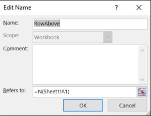
Your cumulative formula in the Table can be entered as =RowAbove + [@Units Sold]]
This works because the N function handles the fact that for the first row the “row above” is the heading and the N turns text to 0
Hope you find this useful!


