Hyperlink Me!
The HYPERLINK Formula (who knew that formula existed?) can be really useful when navigating around large spreadsheets
The simplest format is along the lines of
=HYPERLINK(“#A1″,”Any Helpful Message”)
This would jump you to cell A1 of the current sheet. But that’s no different to a normal old Hyperlink (via RIGHT-CLICK > Hyperlink or Insert > Hyperlink or Ctrl-K)
Where it really comes in handy is if you want to make the link dynamic.
The Dynamic Hyperlink (now we’re getting tricky!)
This is a little complex but….
Lets say you have a very tall spreadsheet made up of different sections. A single formula at the top can allow users to jump to their section of choice (no macros!).
See the example (it uses a match and address formula also but don’t let that put you off, they just combine to give the address of the cell you want to hyperlink to)
The user types or selects a section in cell C3 and then just clicks the hyperlink formula in D3.
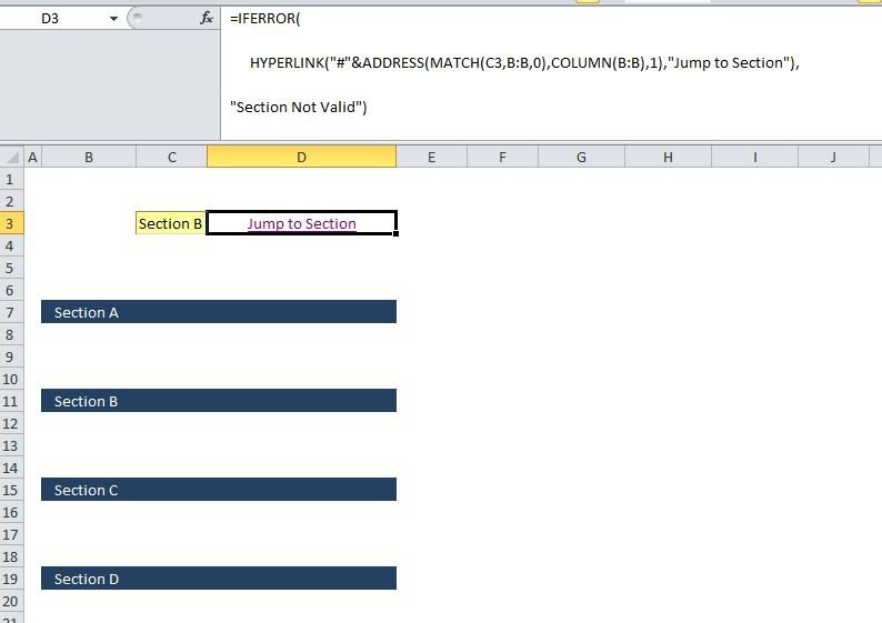
This is the formula:
=IFERROR( HYPERLINK(“#”&ADDRESS(MATCH(C3,B:B,0),COLUMN(B:B),1),”Jump to Section”), “Section Not Valid”)
Note: I’ve wrapped it inside an IFERROR Statement in case the section name selected in C3 does not exist in column B.
Extra example:
Jumping to the bottom of a table
You can use the same approach to create a link to jump to the bottom of a table. For example if someone needs to paste new data each week to the bottom of a list then this quick hyperlink can save a lot of scrolling down…..
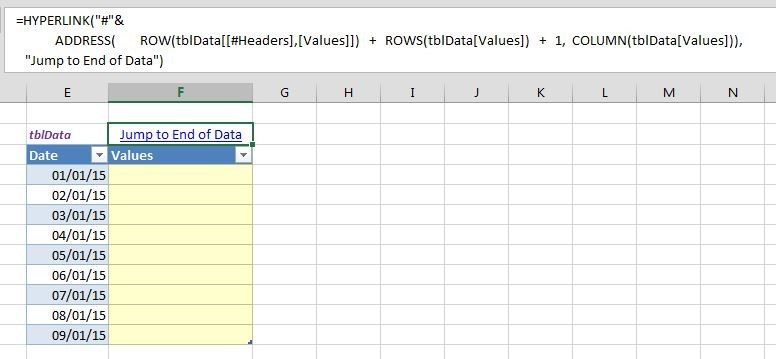
Here is the formula:
=HYPERLINK(“#”&
ADDRESS( ROW(tblData
“Jump to End of Data”)
If that doesn’t make a lot of sense to you, don’t worry! You can always use the simpler versions of HYPERLINK as outlined above.


