
Dynamic Data Validation with Tables in Excel
![]()
Check out our YouTube channel with weekly videos dedicated to Excel, Power Query and Power BI
Why is Excel returning an error message? Why doesn’t my formula work? What did I do wrong?
The answer to these common questions may surprise you.
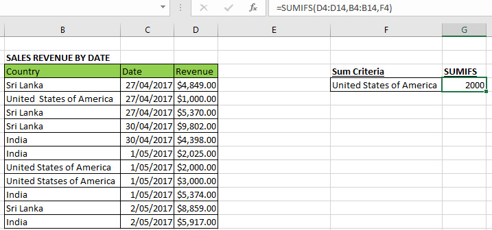
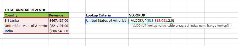
Many spreadsheets I’ve come across have a common problem – inconsistent data entry. If someone enters “United States of America” in a cell, “United States of America ” (extra space after “United” and “America”) in another cell, and then wishes to use “United States of America” as a formula criteria, functions such as SUMIFS and VLOOKUP won’t work properly as “United States of America” was not entered consistently throughout each area of the workbook.
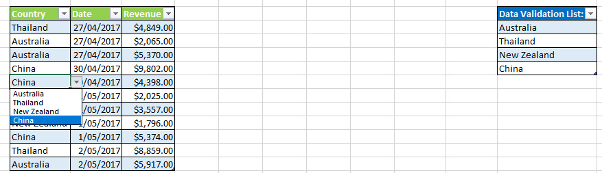
A great way of preventing this problem is to restrict the values that can be inputted into a cell via Data Validation. For example, if your company is currently selling to Australia, Thailand, New Zealand and China, you can enter these values as a list into one section of your workbook, and then use Data Validation to prevent misspelled and other variants of these country names from being entered into a cell.
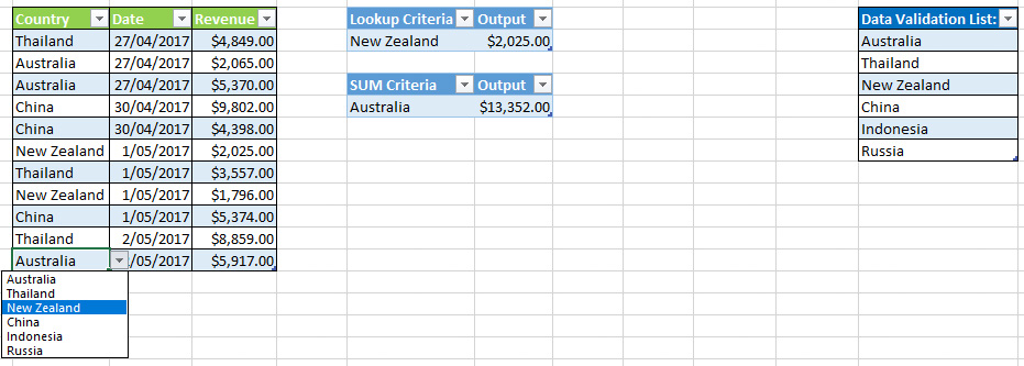
Data Validation is a great tool, but what happens next month if your company starts selling to Indonesia and Russia? How do you automatically extend data validation into subsequent rows of your data entry table to avoid errors? The best way to solve this problem is with dynamic ranges and tables.
Here’s how to do this (file available via the link below to follow along):
![]()
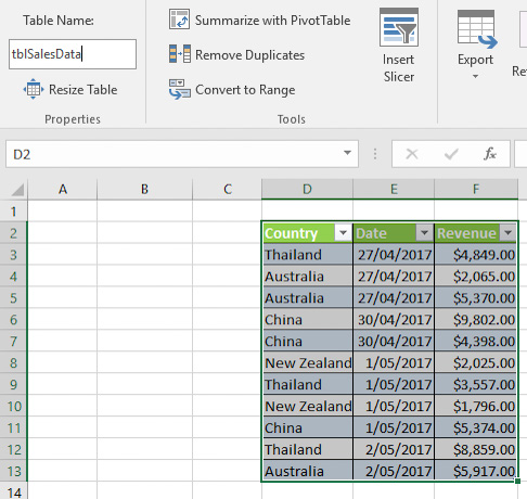
Step 1: Transform Your Data into Tables
If you’ve never used the Excel table feature before, you’re missing out! Excel tables are essential for dealing with large, complicated spreadsheets and help tremendously when dealing with Excel add-ins such as Power Query and Power Pivot.
Begin by selecting your data set (Ctrl + A) and then press Ctrl + T to turn the data into an Excel table. Then click on the Table Name box and give your table a sensible name with no spaces i.e. tblSalesData (“tbl” for Table). Repeat this process for your data validation list.
Step 2: Create a Defined Name
Go to your data validation table and highlight the column that will contain your data validation values (Ctrl + Spacebar). Go to Formulas/Name Manager or Ctrl + F3 to open the Name Manager.
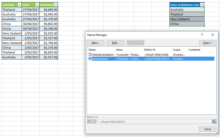
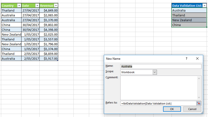
Click the “New” button. Enter an appropriate name, such as ddCountries (dd for “dropdown”). Note that the “Refers to:” box is referring to every item in the data validation column with table formula nomenclature (table name followed by column name in square brackets). Click OK.
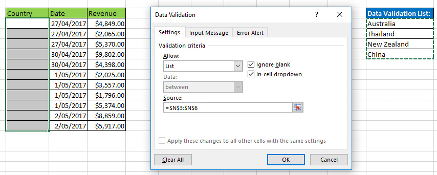
Step 3: Add Data Validation
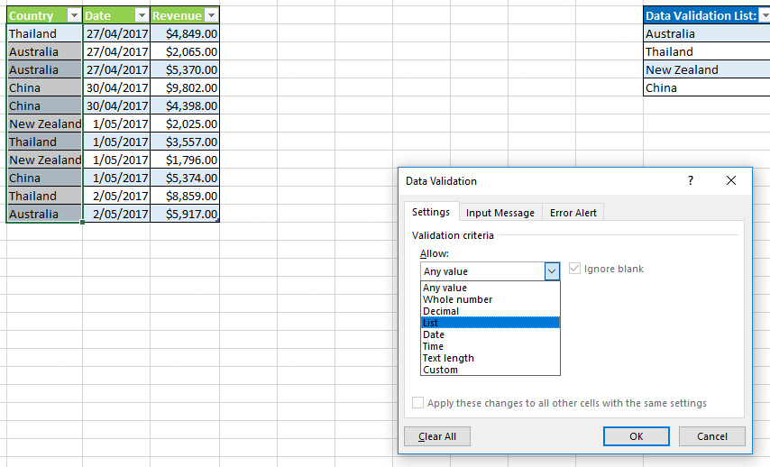
Select the column in your data entry table that you wish to add data validation to. Go to Data/Data Validation or Alt + D + L to open the Data Validation window. Select “List” from the “Allow” dropdown menu.
In the “Source” box, hit the F3 key and select your defined name from the “Paste Name” box. Click OK twice to return to the main screen.
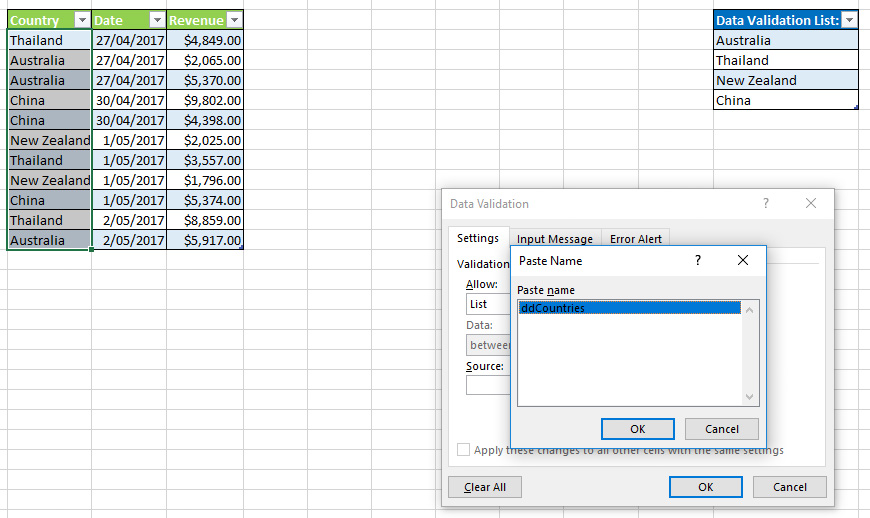
Now every cell in the column will contain data validation that is restricted to the values in the “Data Validation List” column. If you add another row to the Data Validation table, this will automatically appear in the drop down menus you have just created. New rows added to the revenue table will also include data validation for these values by default.
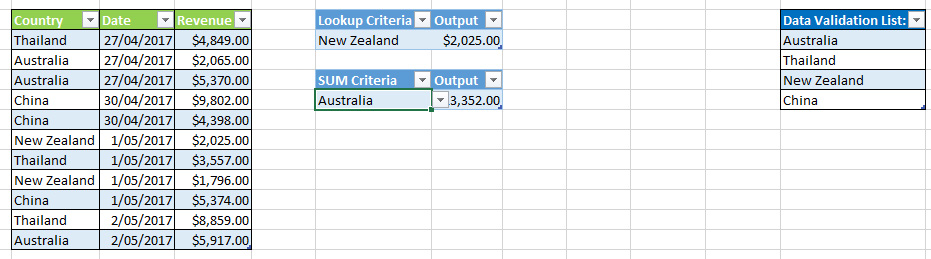
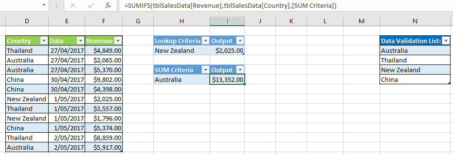
For additional fun, you can add additional tables with data validation to cycle among formula values.
If you found this interesting you may want to explore how to create a dependent validation drop down. Find out how here.


