How to Integrate Excel and Google Maps via PowerQuery
Using the Google Maps API
By Jeff Robson
PowerQuery is indeed a powerful tool for pulling in data from all kinds of different data sources.
More and more websites are making their data available via APIs (Application Programming Interfaces). These are essentially the back-end interfaces that allow programmers to provide all the lovely integration features we all take for granted!
Using PowerQuery, you can now use Excel to get access to the data they make available.
In this example, we show how to use PowerQuery to get the driving times between places via the Google Maps API.
Step by Step
Google Maps API documentation tells us that the syntax for queries is:
http://maps.googleapis.com/maps/api/directions/output?parameters #sthash.QNnv1OZQ.dpuf
Where output is either json or XML, depending on what format you want the results in, and parameters are any of the parameters listed in their documentation.
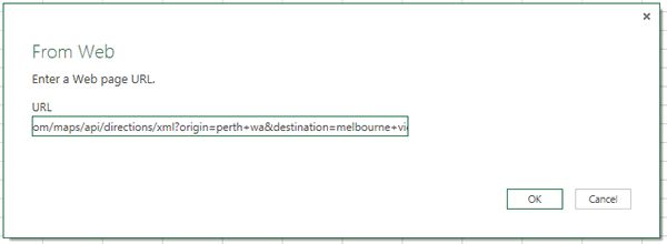
PowerQuery > From Web
Then enter the following URL:
http://maps.googleapis.com/maps/api/directions/xml?origin=perth+wa&destination=melbourne+vic
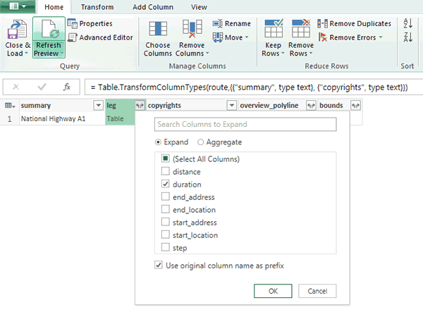
This produces a table which (so far) doesn’t look very useful! Click on the word Table in the route column to drill down.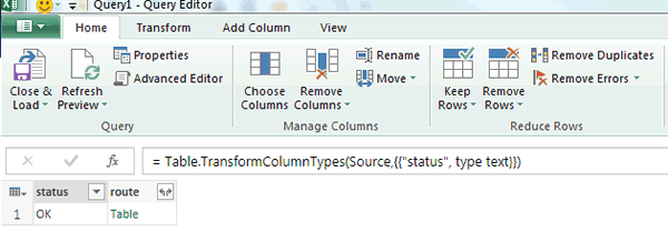
We now need to click on the button highlighted below to choose which parts of the leg column we actually want in our results.
I’ll just choose the duration for this example.
Click OK to select duration, then Table in the leg column to drill into this column.
You should now see a table with one row and 2 columns. The value column shows the estimated driving time in seconds (great for calculating or charting), while the text column shows a much friendlier version of this number.
Right-click on the value column and select Remove to drop this column since we won’t need it for our example.
You should be left with something like this:
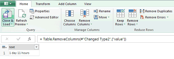
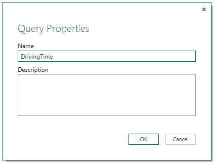
Click the Properties button and change the name to DrivingTime
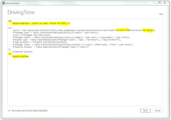
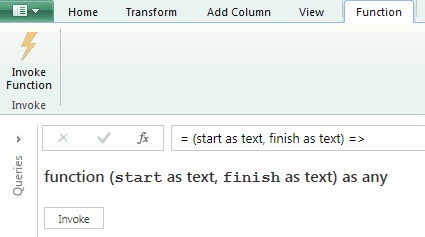
Click the Advanced Editor button and change the code as highlighted below:
You’ve now created a new custom function in PowerQuery that can be applied to other tables.
Click the Green dropdown in the top left-hand corner and choose Close and Load. This will take you back to your workbook with your new function showing under Workbook Queries.
Don’t worry if it says “Load is disabled.” It’s a function so it doesn’t load anything directly into your workbook.
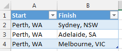
Next, create a table in your workbook with 3 cities you want to measure driving times between. For example:
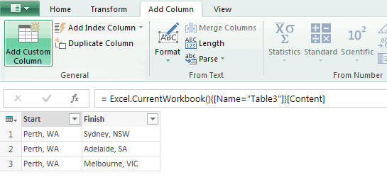
Click a cell within the table, then click the From Table button to import your table of cities into PowerQuery.
Go to Add Column > Add Custom Column
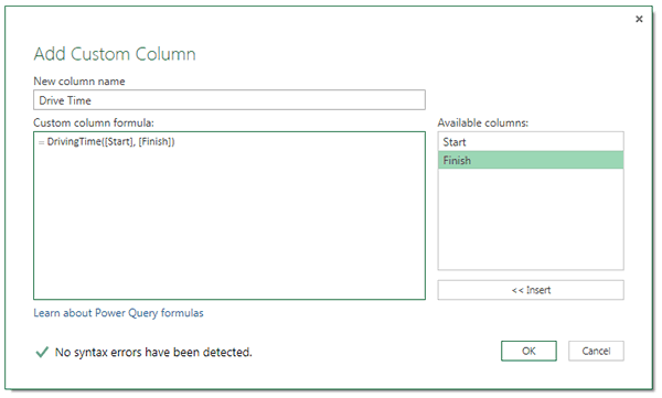
Enter whatever name you want for your new column, then type the formula shown:
=DrivingTime([Start], [Finish])
This will use the values from the Start and Finish columns as inputs for your custom formula.
You may get asked about Privacy. If so, click Continue and make the query Public.
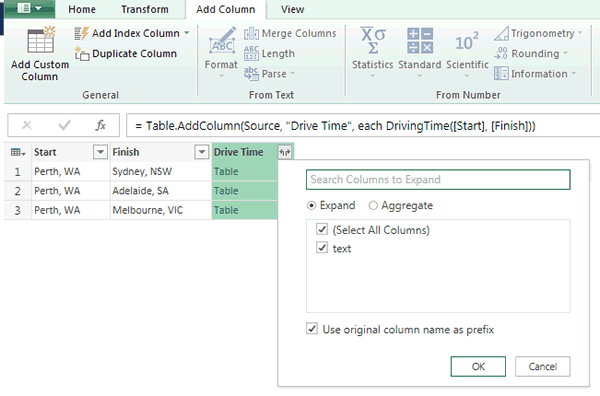
You’ll then see a new Drive Time column and if you expand this, you can access the text column.
The finished product in PowerQuery:
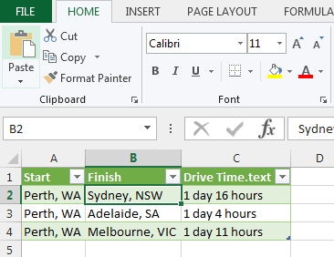
And after you click the green button > Close and Load, you’ll see the same thing in Excel:
Voila! Perth is a REALLY long way from anywhere! Our closest capital city is 28 hours’ drive away!
Warning: don’t try to do this with lots of data! Google specifically limits how many queries you can do per second, even for paying customers.


