The Union All Query

Combining two tables of data into one without Macros

By Wyn Hopkins

 

You may have regular reports that you collate and then manually copy and paste together or you may use macros to combine them together.

But there is another way that, once set up, is very easy to update – a simple right-click and Refresh does all the work for you.

You can then link pivot reports or SUMIFS formula etc to this combined table of data and hey-presto your reports are ready

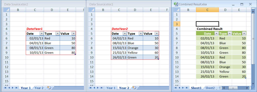
Here’s a step by step guide on how to set this up using a file I’ve called Data Source.xlsx.  In this illustration there’s only 2 tables being combined – year 1 and year 2 but you could add multiple years if required.

Importantly I named my ranges of data first using the Name Manager and then converted them to tables using the Ctrl+T shortcut (creating a table first and then naming the range can make life difficult).

Once you have your source data set up then save the file and close it before proceeding.

Now open a new workbook and follow these steps:
Using Microsoft Query

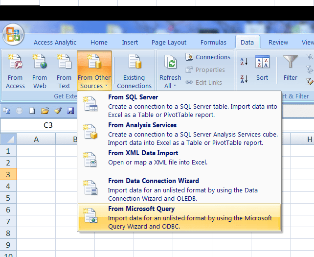
Go to Data, From Other Sources, From Microsoft Query

 

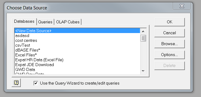
Select New Data Source and click OK

 

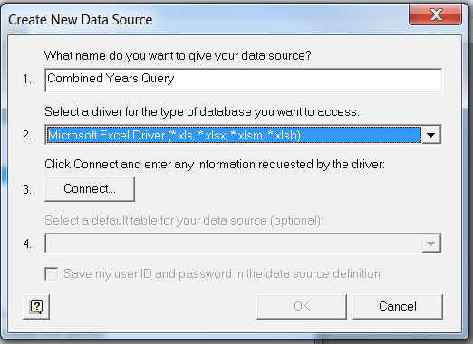
Give it a name and then select Microsoft Excel Driver and click Connect

 

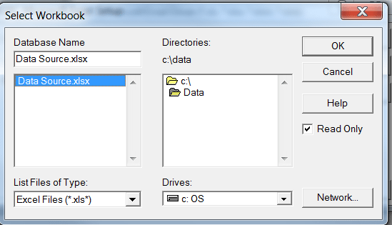
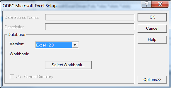
Click on Select workbook

 

And locate your source data file, click on it and click OK

 

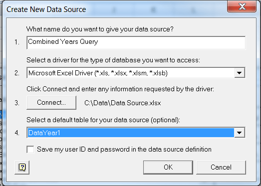
Select the drop down DataYear1 and click OK

 

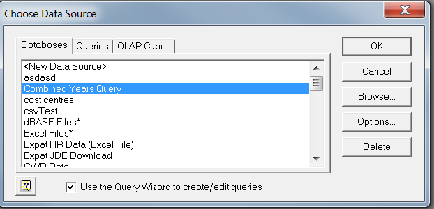
Click on Combined Year Query and select OK

 

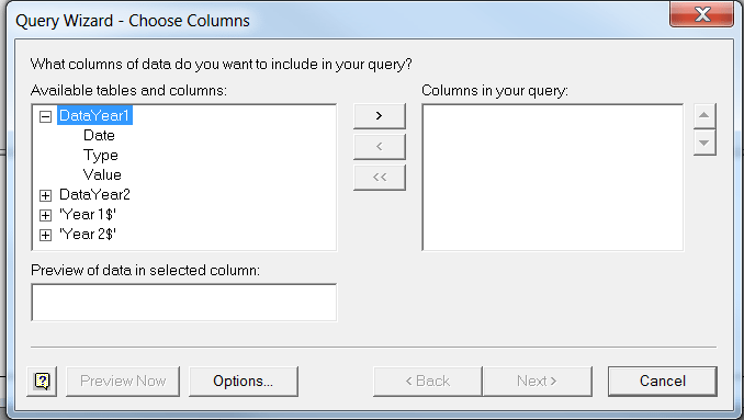
Add both DataYear1 and DataYear2 to the “Columns in your query:” box

 

Click OK

 

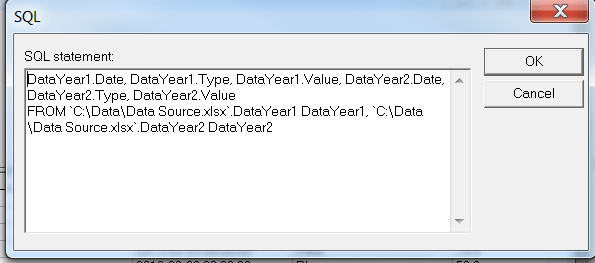
Select View > SQL

 

You should then see something like this…

 

Re-arrange the query to look like this (use Ctrl X and Ctrl V to cut and paste)

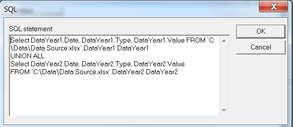
Add the line UNION ALL between the 2 queries

 

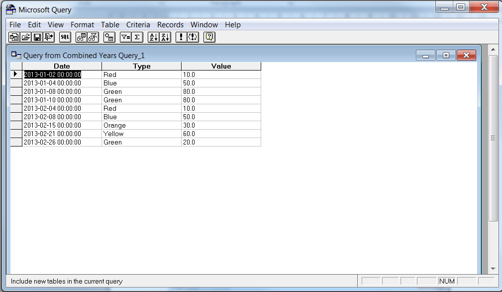
Click on the door with the arrow to return the data to Excel

 

Hey Presto!

 

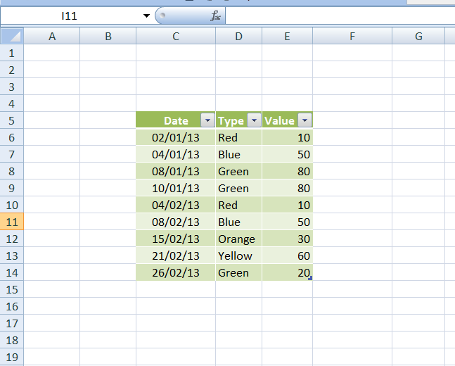
You can then refresh this table at any time by right clicking on it and select Refresh  (or go  to the data menu and select Refresh All).
Any formula columns you add to the table will automatically populate as the data expands (or contracts).