How to Create an Advanced Filter in Excel without Macros
By Simone Palmas
Want to filter your Excel data efficiently without using macros? Filtering data can sometimes feel restrictive, especially when you want to search for multiple words independently of their order or the specific columns they might appear in.
Access Analytic team member, Simone Palmas, has created this handy guide will show you how to filter a table by entering any number of words in a Search box, which will then be searched across the specific columns you choose, regardless of the order.
Creating a single multi-criteria search box to return a filtered view of a table:
This is the table I will filter:
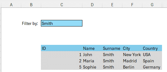
when I search “Smith”, my filtered table will return all the rows from the original table which include the word “Smith”:

If I want to filter the table to get all the rows which include “Smith” and “USA”, independently from the order, I can enter those 2 words to filter the table:

Here’s a step-by-step guide to set it up:
Step 1: Prepare Your Table
1. Create or Import Your Table: Ensure your table is ready and formatted correctly as a table. For this example, I have created a simple table with a list of clients and general information:
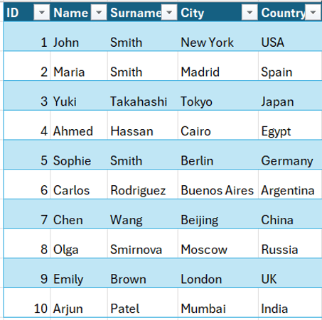
I might want to filter this table by a certain name, surname or country, for example.
Step 2: Set Up the Search Sheet
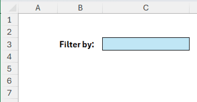
1. Create the Search Box: Decide where you want to enter the words to filter the table and format it to make it clear that it is the input Search Box. I added a new sheet and formatted cell C3 to look like a Search box:
2. Trim and Textsplit the Text in the Filter: Use this formula to return a dynamic array with all the words entered in the Search Box:
=IFERROR(TRIM(TEXTSPLIT(C3,’,’,)), ”)
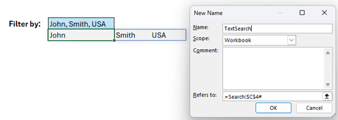
For example, when I type “John, Smith, USA”, the dynamic array will return all these words in separate cells:

After testing it, you can hide or format this row, as you probably do not want to see it.
Note: In this example, words are separated by commas. So, you need to separate each word or phrase by a comma.
3. Assign a Name to the Trimmed Text Dynamic Array: This is an optional step to make the formula easier to understand and improve its Readability.
– Go to Name Manager and create a new name called TextSearch.
– In the “Refers to” field, click on the cell containing the trimmed text (C4 in my case) and add a # at the end, as this is a dynamic array.
Step 3: Add the Search Result Column to Your Table
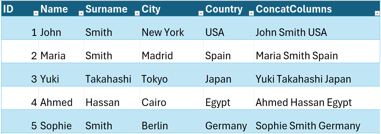
1. Select the sheet which contains your original table and add a new column to concatenate the Columns You Need to Filter. In my example, I want to filter my table by Name, Surname, and Country, so I used the following formula:
=[@Name] & “ “ & [@Surname] & “ “ & [@Country]
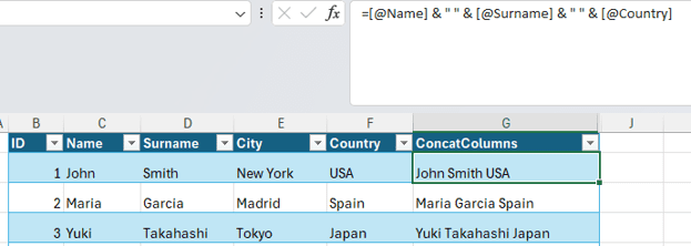
2. Create a new Column to Check if the Searched Words Are Found. Add a new column, I called it: SeachResult.
Then enter the following formula to check if the searched words are in the column you previously created (in my case, ConcatColumns):
=MIN(ISNUMBER(SEARCH(TextSearch, [@ConcatColumns])) * 1) = 1

If you want to understand the logic of this formula, you can read the explanation, or you can go directly to the next step (Step 4).
Explanation of the Formula
The formula performs a multi-step process to determine if all specified words are present in a cell. Here’s how it works:
1. SEARCH: Search for Words:
The SEARCH function returns the position of each word entered in the search cell. If a word is not found, SEARCH generates an error.
For example, let’s consider searching for “Smith” and “USA” within the following rows of data:


In the first row, which contains (1; John; Smith; New York; USA), the ConcactColumn is: “John Smith USA”.
Using the SEARCH function, the results are as follows:
=SEARCH(“Smith”,”John Smith USA”) returns 6 because “Smith” starts at the 6th character, and =SEARCH(“USA”, “John Smith USA”) returns 12 because “USA” starts at the 12th character.
In the second row, which contains:
(2; Jane; Smith; London)
The ConcactColumn is “Jane Smith London”. Here, the SEARCH function results are: =SEARCH(‘Smith”, “Jane Smith London”) returns 7 because “Smith” starts at the 7th
character, and =SEARCH(“USA”, “Jane Smith London”) returns #VALUE! Because “USA” is not found in the text.
2. ISNUMBER: Convert Errors to Logical Values:
The ISNUMBER function is used to convert any errors to FALSE and any other values (positions) to TRUE.

3. _* 1: Convert Logical Values to Numbers:
The formula multiplies the TRUE/FALSE values by 1 to convert them to 1 (for TRUE) or 0 (for FALSE).

4. MIN: Find the Minimum Value:
The MIN function finds the smallest value in the list. If at least one word is not found, the list will contain a 0, making the MIN value 0.
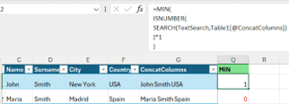
5. _=1 Determine if All Words are Found:
The formula checks if the MIN value is 1. If MIN returns 0, it means at least one word was not found. If MIN returns 1, it means all words were found, and the formula will return TRUE. We want to filter only the rows where all the words are found, hence the ones = TRUE.
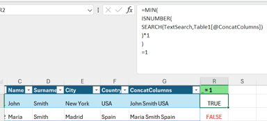
In summary, this formula verifies the presence of all specified words in a cell and returns TRUE if all words are found, allowing you to filter and display only those rows.
Step 4: Set Up the Filter Table
1. Filter the Table: Go back to the sheet with your Search Box, and in a cell beneath it, use the FILTER function to get all the rows in your table that include the searched words. The formula is:
=FILTER(MyTable, MyTable[SearchResult] = TRUE)
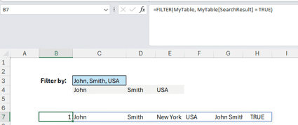
This will return all the rows in your table that include the searched words. Note that the result will not include the headers, which you can easily copy manually from the original Table.
The order of the words won’t change the final result. This is how the table will look after hiding the dynamic array row (4), copying the headers, hiding unused columns, and applying conditional formatting.
By following these steps, you can set up advanced filters in Excel to efficiently search and filter your data based on multiple criteria across various columns. This method is powerful and flexible, allowing you to filter large datasets without using macros and regardless of column order. The key steps involve preparing your table, setting up a dynamic search array, adding a search result column, and finally filtering your table based on these results.


