By Yury Tokarev

Dynamically consolidate multiple ranges when loading Excel files from Folder in Power Query

We’ve come across a task where we need to consolidate a client’s budget data from Excel files, each representing a division, where any of the files may have multiple similarly structured tabs with sub-divisional data. In our project, each subdivision tab contains a local range rng_data, which includes 12 months of forecast data, row headers and column headers. Below is a snapshot of source data:

We are going to use Get Data from Folder to load data into Power Query (Data>Get Data>From File>From Folder). After opening the ‘Combine Files’ dialogue (by clicking ‘Combine & Edit’), we come across the issue that we can only select a single range to combine data from, while the similarly named Excel local ranges get an incremented numbering at the end (as shown on the image below, where the range name for Subdivision B tab gets ‘1’ at the end of ‘rng_data’).

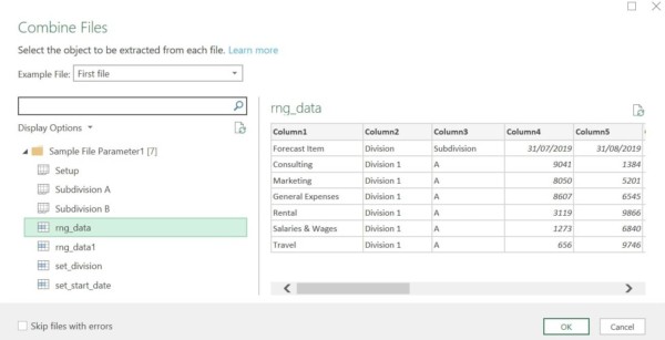
At this stage, let’s select rng_data and click ‘OK’. As a result, Power Query will return consolidated data for Subdivision A (only) in each of the division files.

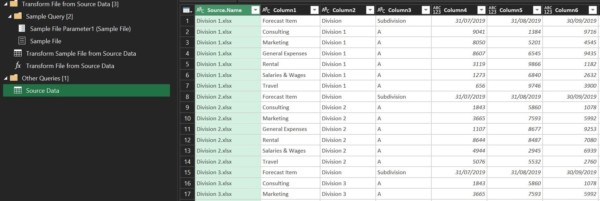
From the Source Data preview window we can see that we need to rectify data headers and unpivot forecast data to show it in one column. We could easily accomplish these tasks in the ‘Transform Sample Files from Source Data’ query by selecting ‘Use First Row as Headers’ and unpivoting columns other than ‘Forecast Item’, ‘Division’ and ‘Subdivision’. However, before doing it, we need to bring in missing data from other subdivisions.

Here are the steps how we can accomplish this:

Step 1: Let’s get rid of the ‘Navigation’ step in the ‘Transform Sample File from Source Data’ query, which will leave us with the ‘Source’ step only.

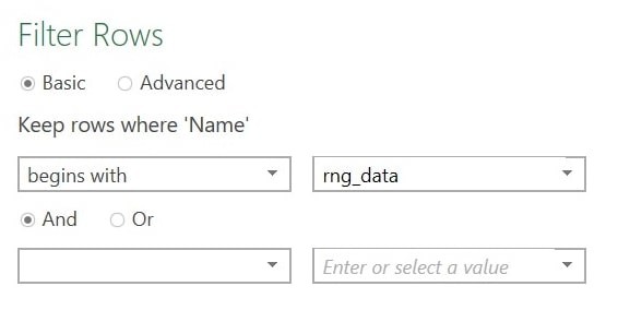
Step 2. In the ‘Name’ column let’s set a filter to show anything beginning with ‘rng_data’

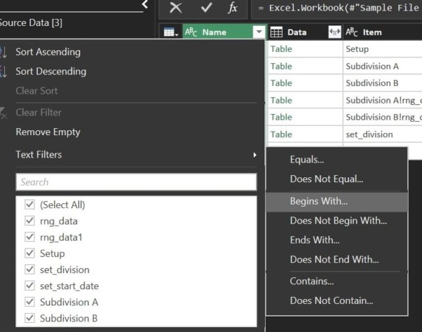
Step 3. Remove all columns apart from ‘Data’ column, which contains source data by selecting ‘Data’ column>right click>’Remove Other Columns’. Rename the step to ‘SourceTables’

Step 4. Expand column ‘Data’ by clicking the arrows pointing sideways as shown in the image below.

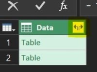
This step returns combined data for all local ranges named ‘rng_data’. However, we can see from the formula bar that the ‘Expanded Data’ step hard-codes column names, which may cause query to break if new columns are subsequently added to the source data.

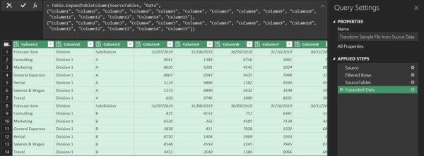
A better approach would be to dynamically generate a list of column names and replace the hard-coded column names with this list.

To achieve this we will apply ideas mentioned by Marc in his recent post ‘Dynamically expanding and appending tables with Power Query’. In particular, we will use Table.ColumnNames function to generate a list of column names in a new column added immediately after the ‘Filtered Rows’ step. We will do it as part of the next step.

Step 5. Select the previous ‘SourceTables’ step in ‘Applied Steps’, then Add Column>Custom Column. Type ‘=Table.ColumnNames([Data])’ in the ‘Custom column formula’ window and click ‘OK’

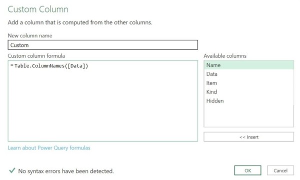
This will add a new column with lists of headers for each table.

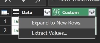
Step 6. Select ‘Expand to New Rows’ at the top of the ‘Custom’ column.

Step 7. Right-click the ‘Custom’ column header, after which we get the following table

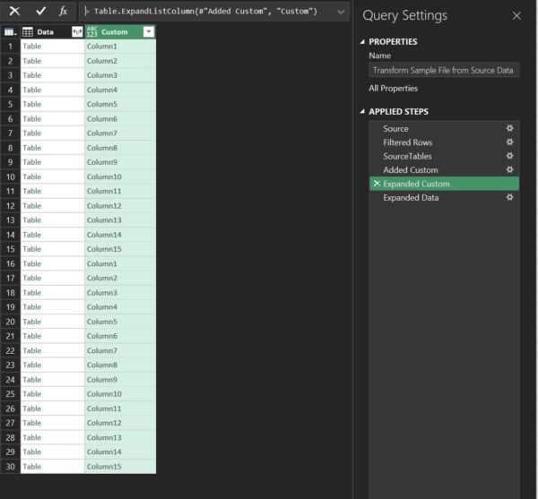
Step 8. Now we need to create a list of column headers, which we can use in the subsequent ‘Expanded Data’ step to substitute the hard-coded column names. The easiest way to create the list is to right click on the ‘Custom’ column header, and select ‘Drill Down’. However, while this action would, helpfully, generate the code ‘#”Expanded Custom”[Custom]’, it would, unhelpfully, wipe away the ‘Expanded Data’ step, where we need to use the newly created list in the first place.

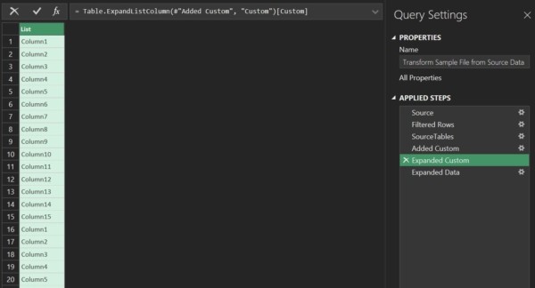
To work around this, we can slightly modify the code in ‘Expanded Custom’. In particular, while having the ‘Expanded Custom’ selected, add ‘[Custom]’ at the end of the code in the formula bar, so that it looks as follows:

= Table.ExpandListColumn(#”Added Custom”, “Custom”)[Custom]

This would generate a list column names. This list, however, contains duplicate values, which we will deal with in the nest step.

Step 9. We assume that the number of columns is exactly the same across all input files, therefore, it is safe for us to remove duplicates from the list. To do so, right-click on the list header and select ‘Remove Duplicates’.

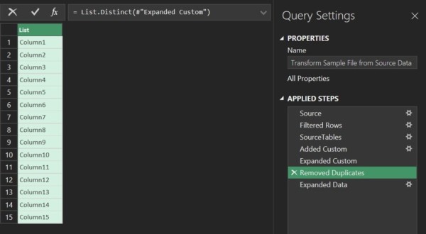
Step 10. Now, we are able to use the list in the ‘Expanded Data’ step. At first, let’s rename the ‘Removed Duplicates’ to ‘ListOfColumnHeaders’ (as shown on the image below) to make it consistent with what the step returns.

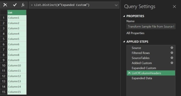
Now is the time to modify the ‘Expanded Data’ step to return data from all ranges of the source files.

At this stage, when you select the step ‘Expanded Data’ in ‘Applied Steps’, you will get the following error message.

This is because it refers to the preceding ‘ListOfColumnHeaders’ step instead of the original table with data in the ‘SourceTables’ step. Therefore, we need to repoint the step to ‘SourceTables’.

At the same time, we want to replace all hard-coded column names with ‘ListOfColumnHeaders’. As a result, we will get the following string of code:

= Table.ExpandTableColumn(#”Filtered Rows”,”Data”,ListOfColumnHeaders)

The step will generate combined data from all divisions in the source excel files:

Since we have replaced the hard-coded values with a dynamic list, any new column additions in the source data will automatically be processed by the query without any errors.

Step 11. Now we can use the first row as headers by selecting Home>Transform>Use First Row as Headers.

Step 12. As we can see, headers are repeated for each local range loaded by the query. Since we have now got correct headers, we can get rid of the other header rows by filtering out ‘Forecast Item’ value in the ‘Forecast Item’ column

Step 13. Last modification in the ‘Transform Sample File from Source Data’ query is to unpivot columns other than ‘Forecast Item, ‘Division’ and ‘Subdivision’. To do so, select the ‘Forecast Item, ‘Division’ and ‘Subdivision’ columns > right click > ‘Unpivot Other Columns’. Subsequently, rename the ‘Attribute’ column name to ‘Date’. Here is a snapshot of data we will have after the modification.

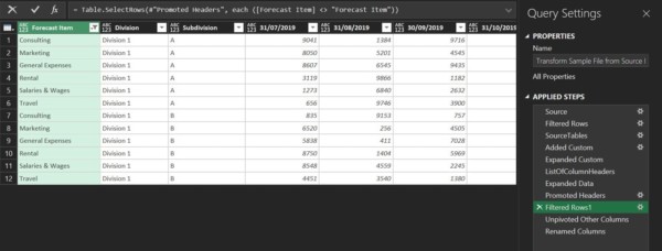
Step 14. Finally, we need to modify the ‘Changed Type’ step in the ‘Source Data’. It would be the easiest to remove the existing ‘Changed type’ step (if it was automatically generated by the query), and recreate a new one manually. This is required as the old ‘Changed Type’ would refer to old columns, which do not exist anymore. The resulting query contains combined data for all divisions and subdivisions form the files saved in our source folder.

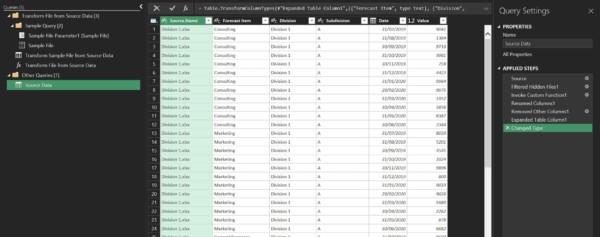
You can download files from the link below if you wish to re-create the steps above, or to have a look at the solution file. Please change the folder path in the ‘Setup’ tab to where you saved the source files.