If you’re not Modelling Depreciation like this, you’re doing it the hard way!

Depreciation is one of those concepts that sounds easy and simple … until you try to put it into a financial model!

In this blog, we start with Excel’s standard depreciation functions, then show two much better, more functional and more elegant ways to calculate depreciation.

1. Excel Functions

Excel has some built-in (although relatively unknown) depreciation functions:

Function	Description	Comments
SLN( cost, salvage, life)	Straight-line depreciation of an asset for one period	A very basic function: ([Cost] – [Salvage]) / [Life] Somewhat useful, although it doesn’t consider the year so it doesn’t know when the asset has been fully depreciated.
DB( cost, salvage, life, period, [month])	Depreciation calculated using the declining balance method	A more sophisticated function that includes a period input so it knows whether the asset is fully depreciated. Excluding the optional [Month] argument, depreciation is calculated as: ([Cost] – [Total depreciation from prior periods] x [rate] Where [rate] = 1 – (([Salvage] / [Cost]) ^ (1 / [Life]))
DDB( cost, salvage, life, period, [month])	Depreciation calculated using the double declining balance method	Similar to the DB function above except that the depreciation is accelerated.

Function

Description

Comments

SLN(
cost, salvage, life)

Straight-line depreciation of an asset for one period

A very basic function:

([Cost] – [Salvage]) / [Life]

Somewhat useful, although it doesn’t consider the year so it doesn’t know when the asset has been fully depreciated.

DB(
cost, salvage, life, period, [month])

Depreciation calculated using the declining balance method

A more sophisticated function that includes a period input so it knows whether the asset is fully depreciated.

Excluding the optional [Month] argument, depreciation is calculated as:

([Cost] – [Total depreciation from prior periods] x [rate]

Where

[rate] = 1 – (([Salvage] / [Cost]) ^ (1 / [Life]))

DDB(
cost, salvage, life, period, [month])

Depreciation calculated using the double declining balance method

Similar to the DB function above except that the depreciation is accelerated.

You can find more help & examples of each in Excel’s Online Help or via Google.

They’re OK for simple calculations but they’re not overly useful and so personally, I’ve never actually used them in a financial model. I’m sure someone must use them however!

2. A Better Straight-Line Function

If you have some assets that are simply being depreciated at x% every year, there is a better way to handle straight-line depreciation than the basic SLN function.

The tricky bit with straight line is that we want Excel to automatically remove those assets that have been fully depreciated, because otherwise they’ll keep on depreciating and we’ll end up with too much depreciation.

Here’s the formula logic for what we really need to do:

[Depreciation Expense] =

[Last year’s depreciation expense]

plus

[Current year’s CAPEX] / [Life]

minus

IF [Year] > [Life] THEN

[CAPEX from [Life] years ago] / [Life]

ELSE

END IF

This effectively removes the CAPEX which has now been fully depreciated from the calculation.

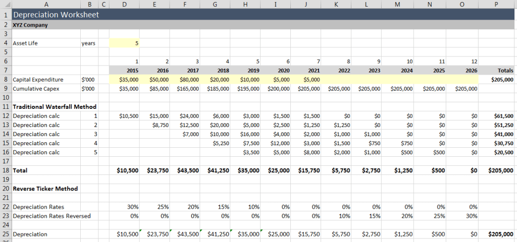
This is what the formulas on row 12 are doing.

Using the OFFSET function, once we get to year 6 and beyond, we remove the depreciation on CAPEX that occurred 5 years ago (since the asset life is 5 years).

Credit and thanks to my friend Damien Beng for this one.

3. Reverse Ticker

The Straight-Line method above works well where there is a consistent depreciation rate. But what about where there is a different rate each year?

The way most financial modellers handle this is to do a separate calculation for each year’s depreciation.

On the first row, the depreciation calculation multiplies the CAPEX in each year by the first year’s depreciation rate (30% in our example).

On the second row, the depreciation calculation multiplies the CAPEX from last year with the second year’s deprecation rate (25% in our example) … and so on until the total number of years has been reached.

This is fine if you only have a small number of rates and small number of asset classes, but it becomes very cumbersome and unwieldy when you have larger numbers of these.

The calculation also has to be manually adjusted for each row – you can’t copy from one row to the next because you must adjust the formula. It’s annoying!

A Better Way

A better way is to use the Reverse Ticker method.

We start by putting all the depreciation rates on a single row, then reversing these using an OFFSET formula (could also be done via an INDEX).

Once we have the rates reversed, we can multiply everything together using SUMPRODUCT that multiplies the CAPEX row (anchored in year 1 and growing by one column to the right each year), with the depreciation rates row (anchored in the final year and growing by one column to the left each year).

The results are shown below: