How to combine multiple tables with Excel Power Query
If you have multiple tables of data in a file and you want to view a single report based on these tables then it can be time consuming and risky to manually copy and paste them into a single table before creating pivot table.
Here’s some steps to do this smoothly with Power Query. I’d recommend downloading the Excel file first so you can step through the process.
![]()
The great advantage of this approach is once you set it up then every future update just requires a single RIGHT-CLICK refresh on the pivot table and hey-presto – immediate update!
The screen shots are from Excel 2016 where Power Query has now been re-labelled as Get & Transform. However, it works in exactly the same way as the Power Query add-in for Excel 2010 + 2013.
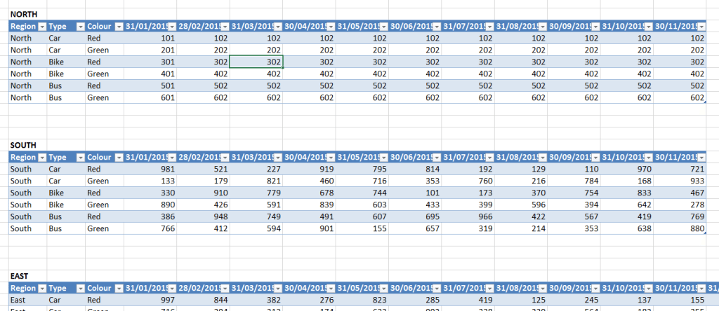
In this example we have 4 tables of monthly data. Each table represents the sales from a different region. We want to combine these 4 tables into a nice easy to manage Pivot Report.
From this…
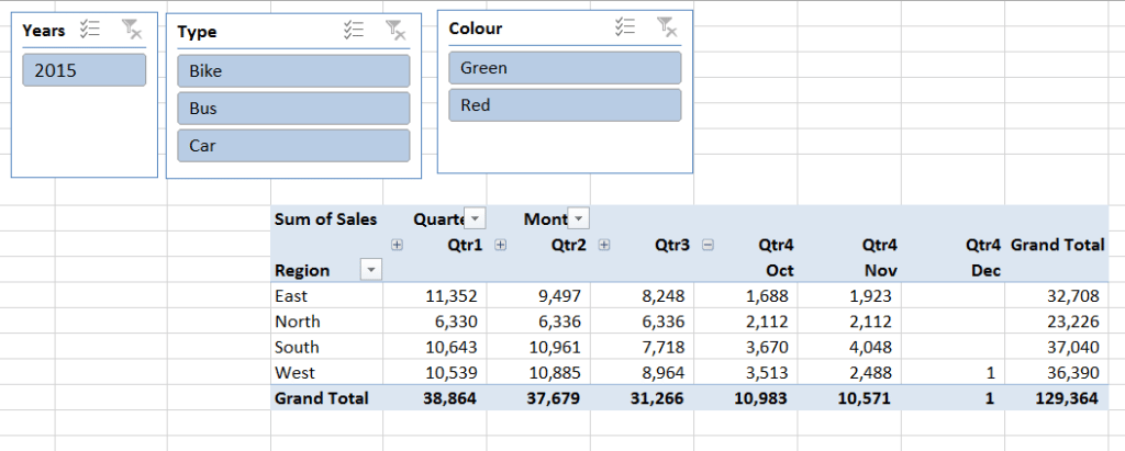
to this….
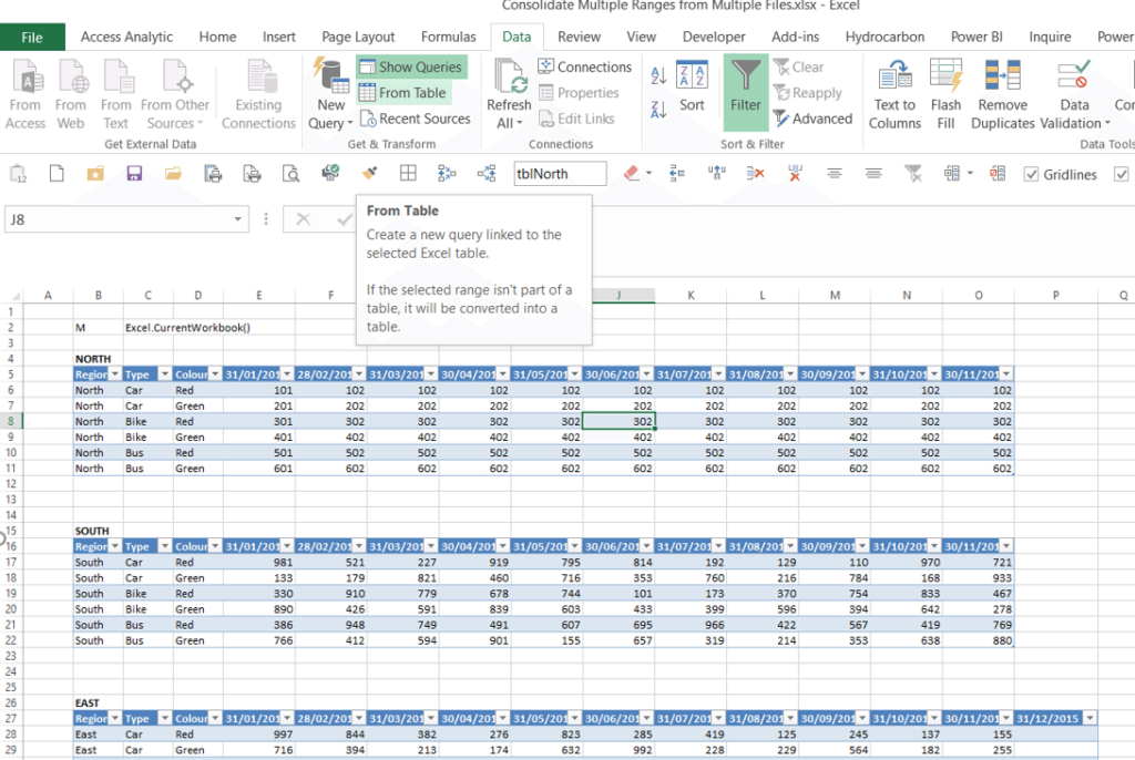
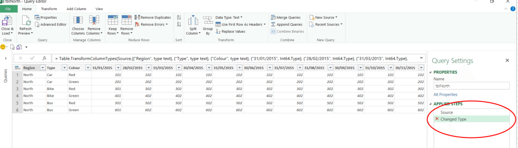
Step 1: Click inside one of the tables (I’ve selected tblNorth) and select Power Query > From Table
Step 2: Delete the Changed Type step
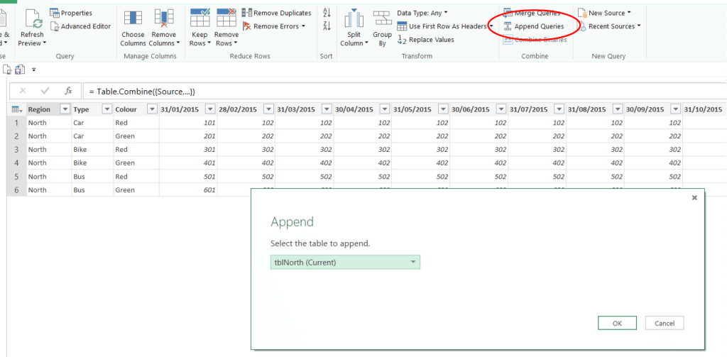
Step 3: Click on Append Queries, and select the current query again. This doesn’t really make sense at this stage as why would you want to append the table to itself? All will be revealed very shortly…
Step 4: This is where it gets interesting, we now need to edit the M code that Power Query has generated for us. This is a bit like stepping into the VBA code after recording a Macro.
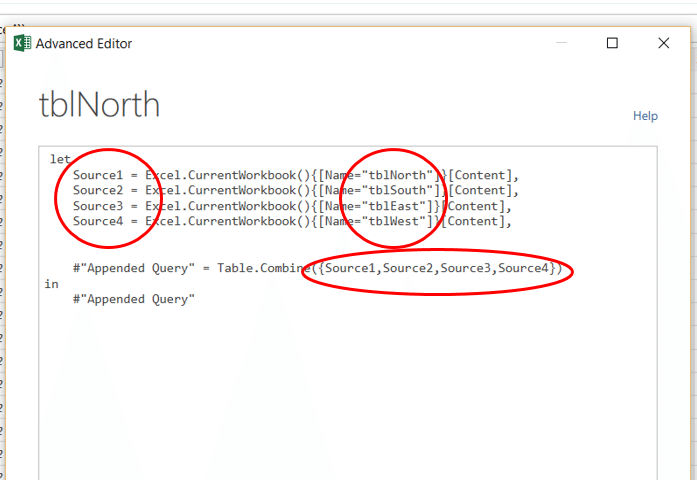
Click on Advance Editor
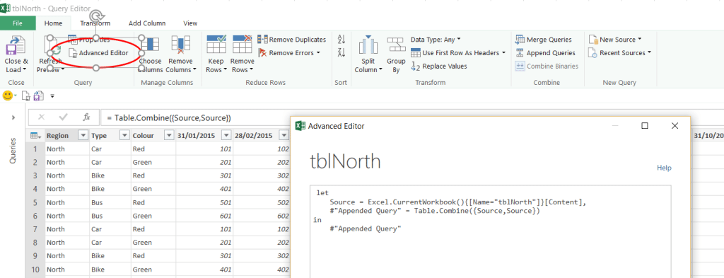
Here’s the code as it stands….
let
Source = Excel.CurrentWorkbook(){[Name=”tblNorth”]}[Content],
#”Appended Query” = Table.Combine({Source, Source})
in
#”Appended Query”
Let’s take a look at this in detail.
Source is just a name that Power Query gave to the data held in tblNorth
The Append function then uses Table.Combine to join Source with Source (i.e. joins the tblNorth data to tblNorth)
We can now use this basic layout to create some “M” Code that can combine all 4 tables in one go…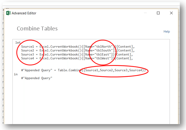
Here’s the amended part
Source1 = Excel.CurrentWorkbook(){[Name=”tblNorth“]}[Content],
Source2 = Excel.CurrentWorkbook(){[Name=”tblSouth“]}[Content],
Source3 = Excel.CurrentWorkbook(){[Name=”tblEast“]}[Content],
Source4 = Excel.CurrentWorkbook(){[Name=”tblWest“]}[Content],
#”Append Query” = Table.Combine({Source1,Source2,Source3,Source4}),
That’s it for amending the M code so we can now click DONE
Step 5: The data from all 4 tables should now be displayed.
If one big table is all you need then you are done and you can skip to step 8. This layout however, with months across the columns, does not work well with Pivot Table reports.
It would be much better if the dates were all in one column. This is where the AMAZING Unpivot functionality comes in.
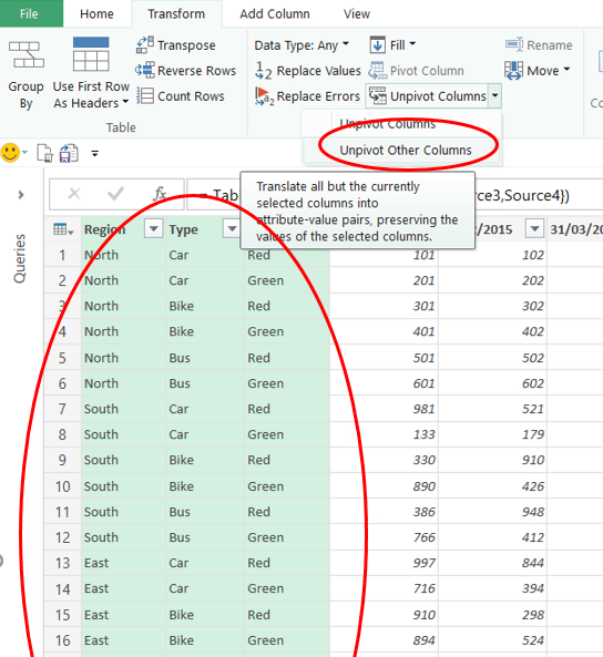
Highlight the first 3 columns (non-date fields) and select Transform > Unpivot Other Columns
How to combine multiple tables with Excel Power Query
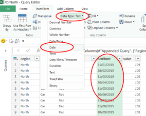
Step 6: All your dates now appear in a new column called Attribute.
Format this as Data Type > Date
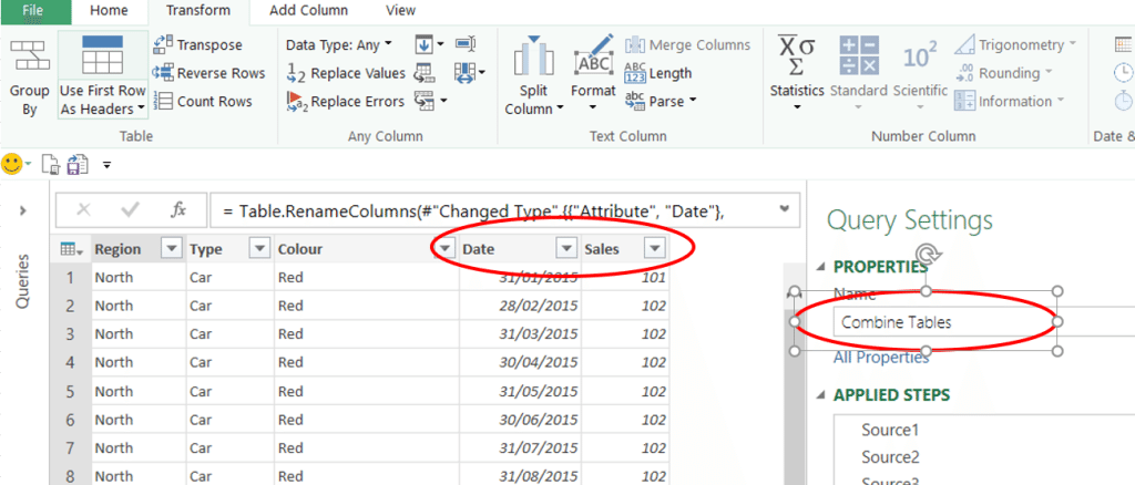
Step 7: Now rename your “unpivotted columns” as Date and Sales, plus rename your Query as Combine Tables
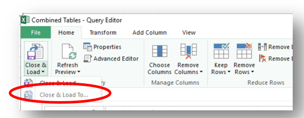
Step 8: At this point you can load your data. Click on the DROPDOWN under Home > Close & Load
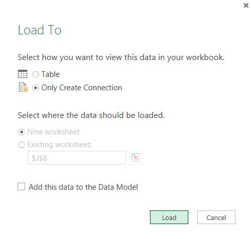
Then choose Close and Load To…
You could load the data to a Table in Excel, or into Power Pivot however here’s one more trick that‘s available. Select Only Create Connection then click Load.
Step 9: We can now access that Query (Connection) directly via a Pivot Table
Go to Insert > Pivot Table
Select Use an external data source (not that it really is external but that’s how this trick works)
Select your Query – Combine Tables

You now have a linked Pivot Table.
Drag Region into rows, Date into columns, Sales into values and then add a few slicers.

Whenever the source tables are updated you can just RIGHT-CLICK on the Pivot table and select Refresh to automatically run Power Query and load this new data.
Author’s comment…
There are several approaches to combining multiple tables, but as of writing (March 2016) this is the most flexible and least error prone approach we’ve identified. Power BI Desktop has recently had an upgrade to allow you to choose multiple tables to append in one go, but until that arrives in Excel we will continue to adopt this approach.


