
by Wyn Hopkins
If you want to create one-off dependent drop-down lists in data validation, you can use a simple technique with XLOOKUP. We did a video on it available here.
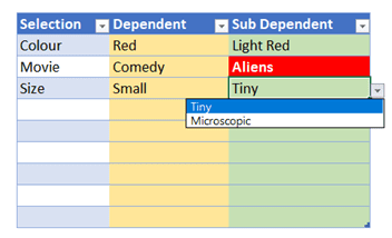
But what if you want to create multiple dependent drop-down lists in a table?
You will need a different approach which many people have done videos on but the solutions were always quite complex or required INDIRECT or many named ranges.
With this technique there’s just 3 formuals
Here are the steps and formulas:
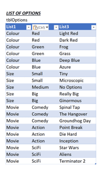
1.Set up the data table with the options for each level of the drop-down list. In this example, I have a table named tblOptions with three columns: List1, List2, and List3. Each column contains the options for each level of the drop-down list.
2.Create some named ranges to store the formulas for each level of the drop-down list. In this example, I have created 2 named ranges: Level1Choice (column G), Level2Result (Column H). You can use any names you like, but make sure they are descriptive and consistent.
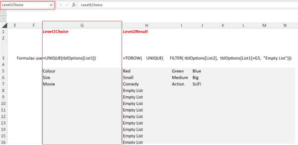
3.Enter the formulas for each named range. Here are the formulas I used:
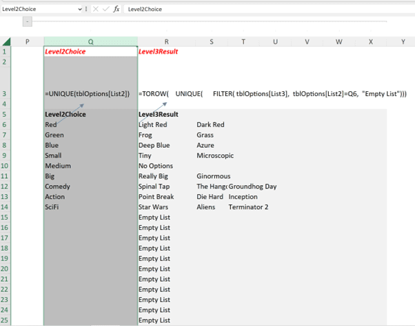
– In G5 of the Level1Choice column: =UNIQUE(tblOptions[List1])
This formula returns the unique values from the List1 column of tblOptions using the UNIQUE function.
– In H5 of the Level2Result colummn: =TOROW(UNIQUE(FILTER(tblOptions[List2],tblOptions[List1]=G5,”Empty List”)))
This formula returns the unique values from the List2 column of tblOptions that match the value in cell G5 (the first level drop-down list) using the FILTER function. If there is no match, it returns “Empty List”. The TOROW function converts the vertical array to a horizontal array for data validation.
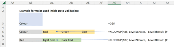
4.Then the magic function is this:
=XLOOKUP( Whatever Cell is to the left of this formula, Level1Choice,Level2Result)#
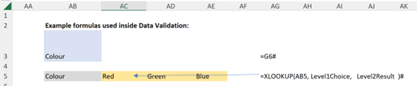
This formula returns the corresponding value from Level2Result based on the value in the cell to the left (in the screenshot above that’s AB5 matching the level 1 selection \ Level2Result is is the named range that contains an array of values and the # at the end allows you to reference that.
I then repeated this process for the next level of dependent drop-downs.
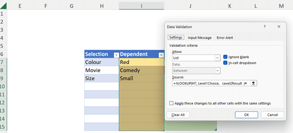
Then set up your selection table and highlight the first column.
Go to Data à Data Validation à List and reference the Unique drop down list in the Level1Choice column – in our case G5# Repeat by highlighting the 2nd column and going to list again and this time enter the XLOOKUP formula in the data validation list source box.
Repeat for Sub-level (note the change to I7 and Leve2Choice and Level3Result.
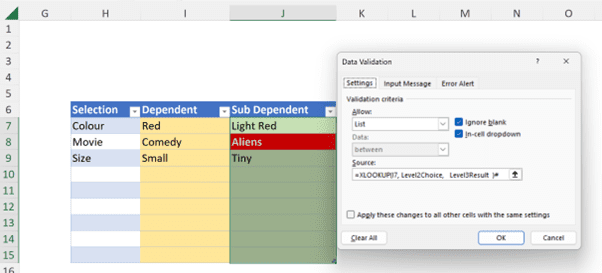
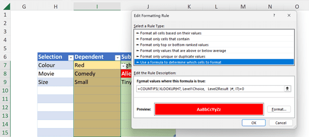
For the conditional formatting I used this formula
=COUNTIFS( XLOOKUP(H7, Level1Choice, Level2Result )#, I7)=0
Which simply checks if the selected value matches an item in the list generated by the XLOOKUP, and then applied a red fill and white font.
Download the file
![]()


